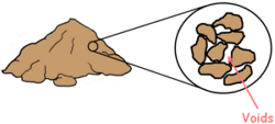
A Soil mass is the huge collection of small particles we call soil grains. These soil grains when depositing in a soil mass encloses empty space between them which we call voids.

 

The water available under the ground moves inside the soil through these voids from the region of high hydraulic head to low head. This phenomenon of flow of water, movement of water through the soil is called seepage.

 

The hydraulic head is the amount of mechanical energy or liquid pressure available at any point in the water above datum.

 

Previously we have considered only uni-dimensional and linear flow of water inside the soil mass but in many soil engineering problems like the flow in the soil under masonry dams is multi-dimensional

As a soil engineer our aim is to analyse the flow of water inside the soil and try to obtain solutions to the engineering problems faced. One such problem is to estimate the quantity of water percolating via seepage through the soil under a dam.

 

To solve such problems and to analyse multi-dimensional flow in soil, we make use of a concept called Flow net. A flow net is a graphical representation of how the hydraulic energy is dissipated as water flows through a pervious medium.

 

To understand the flow net let’s begin with analysing one-dimensional flow before jumping into to multi-dimensional space.

 

Let us consider a soil sample of length L and put it into a glass cylinder. We attach the top of the cylinder with water source and let the water flow through the soil and let it exit from the bottom. We also attach few piezometers at different depths.

 

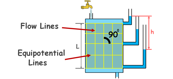
We can observe the flow of water occurs vertically downward under a head difference of say, h. Any water particle that enters into the soil at its top moves vertically downward and the path taken by this water particle can be represented by a line. That line is called flow line.

 

Similarly many particles will flow vertically downward and there will be infinite number of flow lines, but for our convenience we draw only few. These flow lines are also called Stream lines.

 

We can observe that at any level in the soil sample total head is same for all the points lying in that plane. So we can draw a line connecting all the points of equal head. Similarly at different levels such lines of equal heads can be drawn. These lines are known as equipotential lines. All the points on an equipotential line have the same energy.

 

Both of these lines, flow lines and equipotential lines, are crossing each other at right angles and we say they are orthogonal to each other.

We can see these lines form a kind of net and this net is called flow net. A flow net gives a pictorial representation of the path taken by water particles and the head variation along the path.

 

This is a very simple flow net and it is for a uni-directional flow in soil, but for multi-dimensional flow the flow net may be very complex.

Generally the flow of water in soil is three dimensional and analysis of such flow is too complex and difficult. So we simplify the flow situations to two dimensional and analyse the flow.

Then how do we construct a flow net for a two dimensional flow? Well there are some methods for obtaining it.

1. Analytical method

2. Graphical method

3. Electrical flow analogy

4. Capillary flow analogy

5. Sand model

 

We will briefly discuss only first two methods.

 

Analytical method

Analytical method of obtaining a flow net for a flow of water in a soil mass is a mathematical solution to an equation that is obtained by the flow conditions. It can be used in relatively simple cases of flow, where the boundary conditions are known and can be expressed by equations.

 

Let’s consider a soil mass which is completely saturated by water flowing through it. We assume velocity of flowing water in x and z directions are V_x and V_z respectively.

 

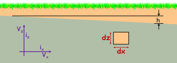
Let us consider a small soil element of dimension dx, dy and dz. y direction is normal to the plane. Let’s say water is flowing in the soil because of a hydraulic head h and the hydraulic gradient in the x and z directions are i_x and i_z respectively. Water is not flowing in y direction as we are analysing flow only in two dimensions.

 

Now using continuity equation we can write the amount of water going in the soil element is equal to the amount of water coming out of it.

 

Somehow after solving it we arrive at simpler equation of continuity.

 

After applying some assumptions like the Darcy’s law is valid we can write velocity of water as permeability times hydraulic gradient.

v = ki

Where permeability in x-direction is k_x hydraulic gradient across this element is i=∂h/∂x

so we can write the equation as :

 

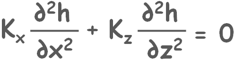
Next assumption is, if soil is isotropic then permeability in x direction is equal to the permeability in z direction.

k_x = k_z

 

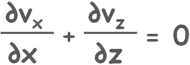
So finally we arrive at this neat and clean partial differential equation.

 

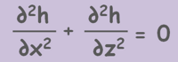
This equation is called Laplace’s equation.

OK. But what do we have to do with this equation. Well, this equation describes the loss of energy through the space and in our case the energy is hydraulic head.

 

When we solve this equation we receive two families of curves. One set of curves is known as flow lines and other set is equipotential lines. Flow lines are also called ψ-lines and equipotential lines are called φ-lines. Once we get these lines, we get our flow net and we can calculate our desired quantities like seepage through soil. But for that first we need to solve the laplace equation, which is not a very easy task to do.

So, we try to obtain our flow net for two dimensional flow using next method.

 

Graphical method

This is the most commonly used method of flow net construction because it is easy and it provides nearly accurate results. This method is one of the solutions to the Laplace equation.

 

Let us understand this method by drawing a flow net for a hydraulic condition.

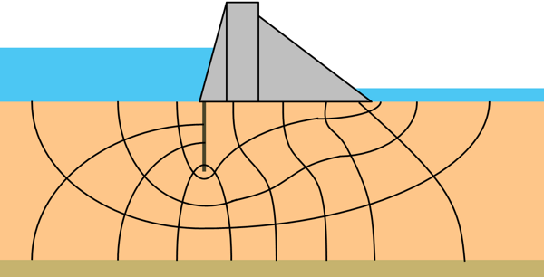
Let's take a soil mass of some thickness and it lies upon an impermeable strata. A sheet pile is driven into the soil up to some depth. The sheet has water on its one side of depth capital D and on another side small d.

We can see there is imbalance of head on the different side of the sheet pile, so water will flow from high head to low head. But water cannot pass through this sheet pile so flow will take place through seepage via soil below.

 

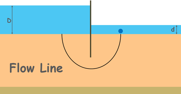
Let us consider a water molecule enters the soil at some point on the upstream surface, goes below the tip of the driven sheet and ends up at some point on the downstream surface. The flow path assumed by a water molecule is the flow line. Similarly many particles will leave the upstream and reach the downstream forming different flow lines.

 

Note that each flow line begins from the upstream surface, which is at pressure γ_wD, and travels through the soil, constantly losing its energy and terminates at the downstream surface, which is at pressure γ_wd.

 

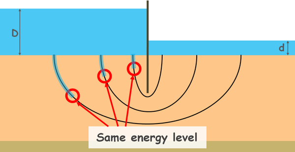
So, we can pick up certain points on the different flow lines where total energy lost is equal, or we can say points of same energy level. When we join such points together, the line so formed is an equipotential line.

 

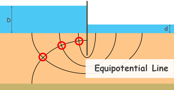
Similarly many different points of the same energy on different flow lines can be observed and many such equipotential lines can be drawn. If we insert piezometers into the soil at different points along an equipotential line we will notice water rises to the same elevation in all these piezometers.

 

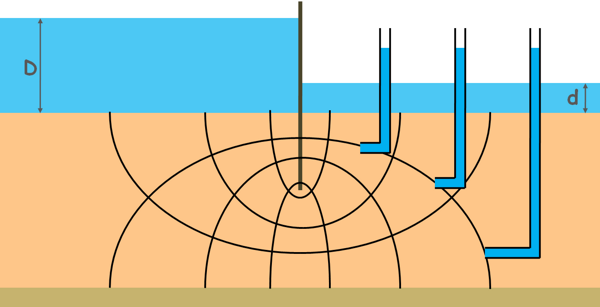
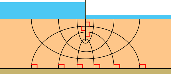
We can see we have received our flow net.

 

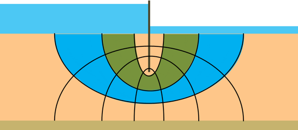
The space between two adjacent flow lines is called the flow path or flow channel.

 

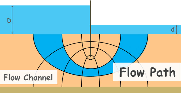
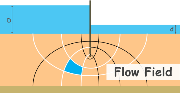
And the area enclosed between any two adjacent flow lines and adjacent equipotential lines is called Flow field.

 

In a flow net we can draw many possible flow lines and equipotential lines, but first it is very inconvenient to draw too many of these lines and second drawing too many lines does not increase the accuracy of the calculations. So, only four or five flow channels are sufficient.

 

To draw a meaningful graph we need to keep in mind certain characteristics of the flow net.

First, two flow lines can never cross each other because flow in soil voids is considered laminar.

Similarly no two equipotential lines can cross each other. Because if they cross at any point then the total head at that point will be two values, which is not possible.

 

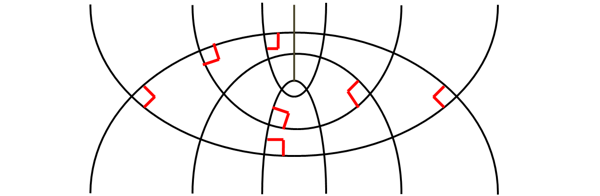
Second characteristic of the flow net is that flow lines and equipotential lines are orthogonal to each other. That means they should intersect each other at right angles.

 

 

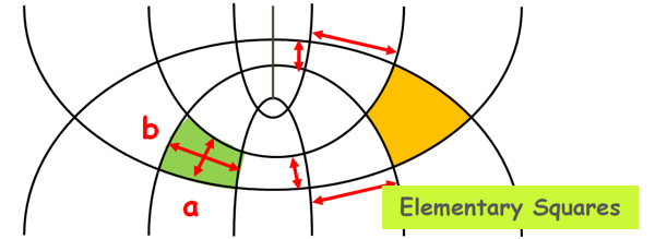
Third, the ratio of the length and width of each flow field (a/b) should be constant.

 

Generally we take this ratio as unity for convenience. In other words, the flow net consists of approximate squares that are called elementary squares. In elementary squares the average distances between opposite sides are equal.

 

To construct a flow net we also need to identify the boundary conditions present for the flow. Boundary conditions are the restrictions that limit the flow in a certain space or area.

 

A flow net is unique for a given set of boundary conditions. If the geometry of the flow space changes, the boundary conditions will be changed and hence the flow net will be changed.

 

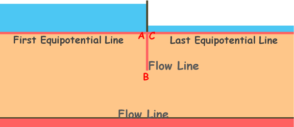
Here, first boundary condition is the upstream surface, from where the flow starts and if we notice, it is the first equipotential line of our flow net as at every point on this line the total head is same.

Second boundary condition is similar and that is the downstream surface, it is the last equipotential line of our flow net.

The third boundary is the sheet pile. Water molecule cannot cross this sheet, it flows from a point which is near to the  sheet on the upstream and moves vertically downward. and after crossing the sheet pile it vertically ascends. The sheet pile is also tracing the flow path of the molecule so this boundary, if we name it ABC, is a flow line.

Fourth boundary is the bottom most impermeable surface. Water molecules cannot cross it. This line is also a flow line as the water will flow along this surface from one side to other.

 

While drawing a flow net we also need to keep in mind that no flow line can intersect the impermeable boundary as the impermeable boundary is itself a flow line. For the same reason all equipotential lines must meet the impermeable boundaries at right angles because impermeable boundaries are flow lines and flow lines meet equipotential lines at right angle.

 

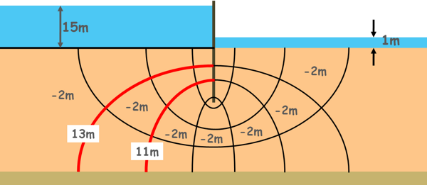
These equipotential lines are drawn in a way that, drop of head or loss of head between two adjacent equipotential lines is constant. Which means if head at the first equipotential line is 15m and after the first equipotential line the head has dropped by 2m so next drop in head should also be 2m and so on.

 

Also the discharge between two adjacent flow channels is constant.

 

Now that we have constructed the flow net its graphical properties can be used to calculate the seepage through soil.

 

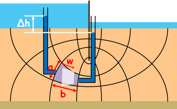
Let’s say height of one flow field is a and length is b.

 

We know from Darcy’s law the discharge through this flow field can be written as this

q = kAi

 

k is the permeability of the soil. A is the area of the cross-section through which the water is flowing. Which is height of the flow field a and its width say w. But it is generally taken as 1 meter.

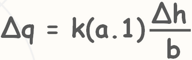
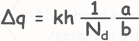
i is the hydraulic gradient which is head loss over the length of the flow field say Δh. So discharge through the flow field can be written as this.

 

Now Δh is the head loss through one flow field, or we can say drop of head or potential drop through one field is Δh, and let’s say there are number of such drops, potential drops is N_d, then total potential drop or head loss through this whole flow channel is N_d times Δh.

h = N_dΔh

 

Let’s substitute this in equation to find the discharge through one flow channel.

 

Note that number of potential drops N_d isnumber of equipotential lines minus one.

N_d = number of equipotential lines – 1

 

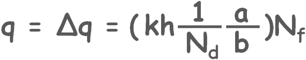
Again this is the discharge through only one flow channel and if total number of flow channels in the flow net are say N_f then total discharge can be written as N_f times discharge through one flow field.

 

Remember that flow net is constructed by elementary squares.

Hence a/b = 1.

So total discharge through soil can be written as this:

 

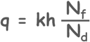
The ratio [Nf/Nd] is called the shape factor.

So this is how we calculate the seepage through soil under any structure using flow net by graphical method.

We know that for a given set of boundary conditions the flow net is unique it is dependent on the boundary conditions. If boundary conditions changes, the flow net will also change.

 

But if we change the soil in which the water is flowing, the flow net will not change. Only the permeability of the soil k will change.

Flow net will also remain unchanged even if the upstream and downstream water levels are reversed; only the direction of the flow will be reversed.

 

We can use the flow net to find solutions to our engineering problems such as the estimation of quantity of seepage losses from reservoirs, determination of seepage pressures, uplift pressures below dams, to check against the possibility of piping and many others.

 

Take a look at an example of this understanding.